2D-Vector Graphics Copyright © by V. Miszalok, last update: 2011-11-14
Let me know what you think	Vertex   Polygon   Length of a polyline   Perimeter of a closed polygon   Area of a closed polygon   Bounding box of a polygon   Center of a polygon   2D polygon scroll   2D polygon zoom   2D polygon rotation   Concentric splash   Bézier Approximation   Cubic Spline Interpolation   Programming curves in parametric form

Vertex

Vertex (latin corner, plural vertices) = vector = point = corner point = POINT is the atomic component of vector graphics. Simplest case: two coordinates containing the two distances from the left and of the upper edge of window.
Alternatives: :
1) 2D-Vertices with 2 float-coordinates:  PointF{ float x; float y; }
2) 2D-Vertices with 2 integer-coordinates: Point { int x; int y; }
3) 3D-Vertices with 3 float-coordinates: Vector3{ float x; float y; float z; }
4) 3D-Vertices such as Vector3 plus color, normal, texture coordinate etc. (see: Direct3D-Vertex Formate)
For 2D-Graphics most often type 1) is used, because this data type permits stepless zoom and rotation and is free from rounding errors.
Simple painting programs use data type 2), because the mouse events supply only integer coordinates and painting instructions like e.g.. DrawLine() require integer coordinates.

Polygon

= most important data type of vector graphics is an ordered quantity of vertices p[0], p[1]... p[i]... p[n-1], whereby the vertices p[i] are connected by lines: DrawLine( p[i], p[i+1] ).
Alternatives:
a) polyline: start- and end-point are not identical. Open polygons have a length, but no perimeter nor area.
b) polygon: start-point identical with end-point. That has the consequence that closed n-polygons have to be coded by n+1 Vertices. A triangle has 4 vertices P0, P1, P2, and P3==P0 ! Closed polygons have a perimeter and an area.
Transformation a) → b): It's possible to close any polyline by copying the no. 0 vertex p[0] to the end of the array.
c) convex polygon: For any arbitrary two points q0 and q1 from the inside: The connecting line segment is fully inside the polygon.
d) concave polygon: There are points q0 und q1 whose connecting line segment is (partly) outside.
e) nonsimple polygon: Intersecting lines occur. Such polygons do not bound a simply connected region in the plane.
Samples:


Order: The vertices are counterclockwise ordered if a traversal of the vertices keeps the bounded region to the left.

Polygons are programmed and stored in the form of arrays.
There are two basic types of 2D-polygon arrays:
a) Polygon as array of fixed length: const Int32 n = 100; PointF[] p = new PointF[n];
Advantage: simple and fast accesses.
Disadvantage: n must be known.
b) Polygon as dynamic array: ArrayList p = new ArrayList(); p.Add( p0 );
Advantage: Simple insert or delete of vertices at any time.
Disadvantages: 1) Namespace using System.Collections; is necessary.
2) Access is slower than with fixed-length array and no access with pointers, because the vertices are not memory-compact, but are stored as a concatenated list.
3) Typecasting = explicit specification of type is necessary (although no conversion of type takes place) on reading from the array: p0 = (PointF)p[i];, because ArrayLists may contain all possible objects in multicolored order.
Tip for painting programs: Store doubly: Collect the vertices first in a dynamic array and copy them later into a fixed array.

Four examples of storage and access of polygons
The following 6 declarations apply to all 4 examples:
using System.Collections; //contains ArrayList
const Int32 n = 100; //length of fixed array
Random r = new Random(); //random generator to fill the arrays
Int32 i;
Pen mypen = new Pen( Color.Red, 1 );
Graphics g = this.CreateGraphics();

1) Example: Point-array of fixed length with integer coordinates
   Point[] p = new Point[n];
   for ( i=0; i < n; i++ ) //write into array
   { p[i].X = r.Next(100); p[i].Y = r.Next(100); }
   for ( i=0; i < n-1; i++ ) //read from array
     g.DrawLine( mypen, p[i], p[i+1] );

2) Example: Point-dynamic array of variable length with integer coordinates
   ArrayList p = new ArrayList();
   for ( i=0; i < n; i++ ) //write into array
     p.Add( new Point( r.Next(100), r.Next(100) ) );
   for ( i=0; i < p.Count-1; i++ ) //read from array
     g.DrawLine( mypen, (Point)p[i], (Point)p[i+1] );

3) Example: PointF-array of fixed length with float coordinates
   PointF[] p = new PointF[n];
   for ( i=0; i < n; i++ ) //write into array)
   { p[i].X = 100f*(Single)r.NextDouble(); p[i].Y = 100f*(Single)r.NextDouble(); }
   for ( i=0; i < n-1; i++ ) //read from array
   { Int32 x0 = Convert.ToInt32( p[i  ].X );
     Int32 y0 = Convert.ToInt32( p[i  ].Y );
     Int32 x1 = Convert.ToInt32( p[i+1].X );
     Int32 y1 = Convert.ToInt32( p[i+1].Y );
     g.DrawLine( mypen, x0, y0, x1, y1 );
   }

4) Example: PointF-dynamic array of variable length with float coordinates
   ArrayList p = new ArrayList();
   for ( i=0; i < n; i++ ) //write into array
     p.Add( new PointF( 100f*(Single)r.NextDouble(), 100f*(Single)r.NextDouble() ) );
   for ( i=0; i < p.Count-1; i++ ) //read from array
   { Int32 x0 = Convert.ToInt32( (PointF)p[i  ] ).X );
     Int32 y0 = Convert.ToInt32( (PointF)p[i  ] ).Y );
     Int32 x1 = Convert.ToInt32( (PointF)p[i+1] ).X );
     Int32 y1 = Convert.ToInt32( (PointF)p[i+1] ).Y );
     g.DrawLine( mypen, x0, y0, x1, y1 );
   }

Length of a polyline

A dynamic vertex array is given: ArrayList p = new ArrayList(); filled with objects of type Point
We want to know Double length;
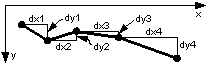
We use the Pythagorean theorem: In the right triangle the hypotenuse is equal to the root of the sum of the squares of the legs. The sum of all hypotenuses is the overall length.
Double length = 0.0;
Point p0 = (Point)p[0];
for ( Int16 i=1; i < p.Count; p++ ) //loop doesn't start at 0 !
{ Point p1 = (Point)p[i];
  Double dx = p1.X - p0.X; //horizontal leg
  Double dy = p1.Y - p0.Y; //vertical leg
  length += Math.Sqrt( dx*dx + dy*dy ); //hypotenuse
  p0 = p1;
}

Perimeter of a closed polygon

A dynamic vertex array is given: ArrayList p = new ArrayList(); filled with objects of type Point
We want to know Double perimeter;
At first let's copy the start point of the polygon to its tail, if this is not the case already.
Double perimeter = 0.0;
Point p0 = (Point)p[0];
if ( p0 != (Point)p[p.Count-1] ) p.Add( p0 ); //close polygon
for ( Int16 i=1; i < p.Count; p++ ) //loop doesn't start at 0 !
{ Point p1 = (Point)p[i];
  Double dx = p1.X - p0.X; //horizontal leg
  Double dy = p1.Y - p0.Y; //vertical leg
  perimeter += Math.Sqrt( dx*dx + dy*dy ); //hypotenuse
  p0 = p1;
}

Area of a closed polygon

A dynamic vertex array is given: ArrayList p = new ArrayList(); filled with objects of type Point
We want to know Double area;
At first let's copy the start point of the polygon to its tail, if this is not the case already.
Double area = 0.0;
Point p0 = (Point)p[0];
if ( p0 != (Point)p[p.Count-1] ) p.Add( p0 ); //close polygon
for ( Int16 i=1; i < p.Count; p++ ) //loop doesn't start at 0 !
{ Point p1 = (Point)p[i];
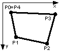
  Double dx = p1.X - p0.X; //width of trapezoid
  Double my = (p1.Y + p0.Y) / 2.0; //average y-value
  area += dx * my; //area of trapezoid
  p0 = p1;
}

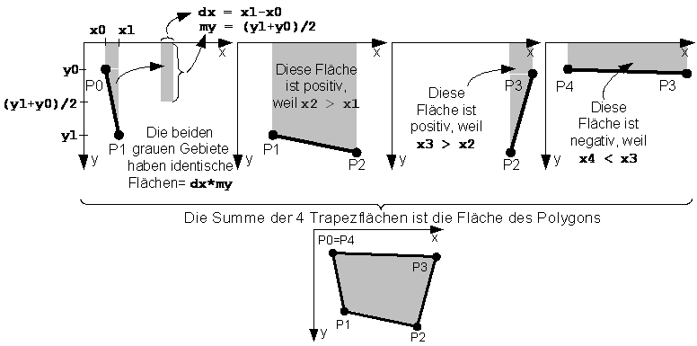
Area can result in a negative value. Its sign depends on the direction of rotation. If the area lies left from the border line (counterclockwise orientation), the area will be positive, otherwise negative. If the result should be independent of the orientation and positive, then write behind the loop:
area = Math.Abs( area );

Bounding box of a polygon

= smallest axis-parallel prison of a polygon. It replaces the polygon in questions whether the mouse is over or if two polygons collide.
A dynamic vertex array is given: ArrayList p = new ArrayList(); filled with objects of type Point
We want to know Rectangle box; //bounding box;
At first we set the four walls of the prison xmin, ymin, xmax, ymax at the start point fo the polygon.

Int32 xmin, ymin, xmax, ymax;
xmin = xmax = ( (Point)p[0] ).X;
ymin = ymax = ( (Point)p[0] ).Y;
for ( int i=1; i < p.Count; i++ )
{ Point p0 = (Point)p[i]          //next vertex
  if ( p0.X < xmin ) xmin = p0.X; //move the left wall to the left
  if ( p0.X > xmax ) xmax = p0.X; //move the right wall to the right
  if ( p0.Y < ymin ) ymin = p0.Y; //raise the upper wall
  if ( p0.Y > ymax ) ymax = p0.Y; //sink the lower wall
}
box = new Rectangle( xmin, ymin, xmax-xmin, ymax-ymin );

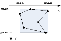Remark: In the class Rectangle the properties X und Y exist also under the names Left und Top. In the example: xmin = box.X = box.Left und ymin = box.Y = box.Top.

Determining collisions is difficult if the polygons have complicated forms. It is much simpler to detect the collision of the bounding boxes. Example:
A moveable rectangle is given: Rectangle box and an array of stationary rectangles Rectangle[] boxes = new Rectangle[n];.
Question: Is box colliding with somebody ?

Solution step by step:
for ( int i=0; i<n; i++ )
{ if ( box.X > boxes[i].X + boxes[i].Width  ) continue; //box is too right
  if ( box.Y > boxes[i].Y + boxes[i].Height ) continue; //box is too low
  if ( boxes[i].X > box.X + box.Width       ) continue; //box is too left
  if ( boxes[i].Y > box.Y + box.Height      ) continue; //box is too high
  Debug.WriteLine( "box collided with " + i.ToString() + ".\r\n" );
}
Solution with the Rectangle.IntersectsWith - method:
for ( int i=0; i<n; i++ )
  if ( box.IntersectsWith( boxes[i] ) ) Debug.WriteLine( "box collided with " + i.ToString() + ".\r\n" );

In mouse events the graphic objects are replaced in the same way by their bounding boxes.
Example: Is the mouse e.X, e.Y inside a graphic object i with the bounding box boxes[i] ?

Solution with the Rectangle.Contains - method:
for ( int i=0; i<n; i++ )
  if ( boxes[i].Contains( e.X, e.Y ) ) Debug.WriteLine("The mouse points at " + i.ToString() + ".\r\n" );

Addendum: See: www.ecse.rpi.edu/Homepages/wrf/Research/Short_Notes/pnpoly.html
1970 Randolph Franklin published the following ingenious algorithm to find out if a point x,y lies inside a polygon p (not only inside its bounding box):

int point_in_polygon(int n, float xp[], float yp[], float x, float y) //p → arrays xp[n],yp[n]
{ int i, j, c = 0;
  for (i = 0, j = n-1; i < n; j = i++)
    if ((((yp[i] <= y) && (y < yp[j])) || ((yp[j] <= y) && (y < yp[i]))) &&
        (x < (xp[j] - xp[i]) * (y - yp[i]) / (yp[j] - yp[i]) + xp[i])) c = !c;
  return c; //c=-1 → x,y is outside; c=0 → x,y is on an edge; c=1 → x,y is inside
}

Center of a polygon

It is better to use float-coordinates (type PointF) instead of integer-coordinates (type Point), since the computation of the midpoint requires a division which seldom furnishes an integer.
There are four definitons of midpoints mp, which can be far away from each other:

2D polygon scroll

Given:
1) a polygon vertex count: const Int32 n = 100;
2) PointF pold = new PointF[n];
3) PointF pnew = new PointF[n]; //result
Operation:
2D-Scroll = 2D-Translation with Single dx, dy.
for ( i=0; i < pold.Count; i++ )
{ pnew[i].X = pold[i].X + dx;
  pnew[i].Y = pold[i].Y + dy;
}
We can do it with one polygon:
for ( i=0; i < p.Count; i++
{ pold[i].X += dx;
  pold[i].Y += dy;
}

2D polygon zoom

Operation: 2D-Zoom = 2D-Scaling with Single zoomx, zoomy.
The polygons pold and pnew must have float-coordinates (type: PointF).
for ( i=0; i < pold.Count; i++ )
{ pnew[i].X = pold[i].X * zoomx;
  pnew[i].Y = pold[i].Y * zoomy;
}
We can do it with one polygon:
for ( i=0; i < p.Count; i
{ pold[i].X *= zoomx;
  pold[i].Y *= zoomy;
}
zoomx < 1.0f = makes a scale down and a shift to the left
zoomy < 1.0f = makes a scale down and a shift upward
zoomx > 1.0f = makes a scale up and a shift to the right
zoomy > 1.0f = makes a scale up and a shift downward
Example:

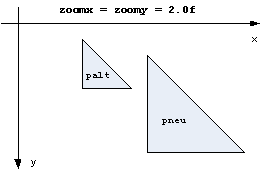
In most cases the shifts are unwanted, since one wants to zoom on place.
For this purpose a midpoint mp is needed:
1) Shift the polygon until its midpoint mp lies on the origin.
2) Zoom around the origin.
3) Back shift.

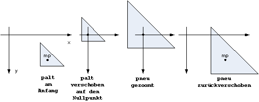
for ( i=0; i < pold.Count; i++ )
{ pnew[i].X = (pold[i].X - mp.X) * zoomx + mp.X;
  pnew[i].Y = (pold[i].Y - mp.Y) * zoomy + mp.Y;
}
We can do it with one polygon:
for ( i=0; i < pold.Count; i
{ pold[i].X -= mp.X;
  pold[i].Y -= mp.Y;
  pold[i].X *= zoomx;
  pold[i].Y *= zoomy;
  pold[i].X += mp.X;
  pold[i].Y += mp.Y;
}

2D polygon rotation

Operation: 2D-Rotation clockwise with Single alpha or Double alpha.
Rotation axis of the 2D-Rotation is the invisible Z-Axis, which pierces perpendicularily the display in the left upper corner of the client area.
The polygons pold und pnew must have float coordinates (type: PointF).
Double arcus = alpha * 2.0 * Math.PI / 360.0; //alpha in radian measure
Single cosinus = (Single)Math.Cos( arcus );   //cosinus(alpha) as float
Single sinus   = (Single)Math.Sin( arcus );   //  sinus(alpha) as float
for ( i=0; i < pold.Count; i++ )
{ pnew[i].X = pold[i].X * cosinus - pold[i].Y * sinus;
  pnew[i].Y = pold[i].X * sinus + pold[i].Y * cosinus;
}
We can do it with one polygon, but we need a help variable, since pold[i].X is needed twice:
for ( i=0; i < p.Count; i++ )
{ Single help = pold[i].X * cosinus - pold[i].Y * sinus;
  pold[i].Y   = pold[i].X * sinus + pold[i].Y * cosinus;
  pold[i].X   = help;
}
If you want to rotate counterclockwise, exchange the signs between both sinus-products:
for ( i=0; i < pold.Count; i++ )
{ pnew[i].X =  pold[i].X * cosinus + pold[i].Y * sinus;
  pnew[i].Y = -pold[i].X * sinus + pold[i].Y * cosinus;
}
Example 90 degrees: pnew disappears from the window by its rotation to the left.

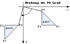
Warning: Similar to 2D-zoom each 2D-rotation is linked with a shift, which nearly never is wanted.
If you want to rotate in place, you have to shift as we did before and after zooming:
1) Shift the polygon until its midpoint mp lies on the origin.
2) Rotate around the origin.
3) Back shift.
for ( i=0; i < pold.Count; i++ )
{ Single x = pold[i].X - mp.X;
  Single y = pold[i].Y - mp.Y;
  pnew[i].X = x * cosinus - y * sinus + mp.X;
  pnew[i].Y = x * sinus + y * cosinus + mp.Y;
}


Concentric splash

= pencil of lines, where all lines start from a midpoint and all endpoints are distributed evenly on a circle.
Given:
1) midpoint: Point mid = new Point();
2) radius: Double radius = 100;
3) number of rays of the star: Int16 const nn = 120;
4) color and thickness of the rays: Pen mypen = new Pen( Color.Red, 5 );
5) end cap of the lines: cut, rounded, arrow etc:
   mypen.EndCap = System.Drawing.Drawing2D.LineCap.DiamondAnchor;
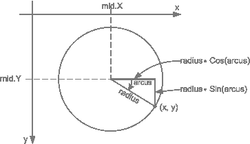
Knowing the angle arcus of a ray (in radian) one obtain x,y using the so called parameter formula of the circle:
x = mid.X + radius * Math.Cos( arcus );
y = mid.Y + radius * Math.Sin( arcus );

The angle in degrees between two adjacent rays is 360.0 / nn, the same angle in radian measure is:
Double arcus_1 = 2.0 * Math.PI / nn;
We need memory space for nn endpoints:
Point[] star = new Point[nn];
and fill this array with the loop:
for ( Int16 i=0; i < nn; i++ )
{ Double arcus_i = arcus_1 * i;
  Double x = radius * Math.Cos( arcus_i );
  Double y = radius * Math.Sin( arcus_i );
  star[i].X = mid.X + ConvertToInt32( x );
  star[i].Y = mid.Y + ConvertToInt32( y );
  g.DrawLine( mypen, mid.X, mid.Y, star[i].X, star[i].Y );
}

Bézier Approximation

Problem: Polygons are awkward (when their vertices are connected by straight lines) but real world objects mostly have smoothly curved borders.
Consequence: Its often better to use curves instead of straight lines and to allow the curves to bypass some vertices rather than to exactly meet all of them.
A very popular solution has been developed 1962 by Pierre Bézier and Paul de Casteljau who use polynomials of degree n-1 to approximate polygons with n vertices.
see: Wikipedia: Bézier curve

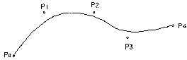Sample with n = 5: The Bézier curve starts at p[0] of the polygon and ends at p[4]. The curve bypasses p[1], p[2] and p[3]. These vertices just provide attraction information and influence the local curvatures.

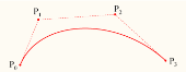Sample with n = 4: A cubic Bézier curve (= polynomial of degree 3 = parabola of type y = a3*x3 + a2*x2 + a1*x + a0 covers 4 vertices. see: Living Math Bézier applet

Piece by piece approximation
In many cases there is no need to cover the complete polygon from p[0] to p[n-1] by a Bézier curve of degree n-1. Piece by piece approximation with sharp edges between the pieces is a widely used alternative. True Type Fonts TTF outline their characters in such a way with quadratic polynomials that cover 3 vertices. PostScript makes the same with cubic polynomials that cover 4 vertices

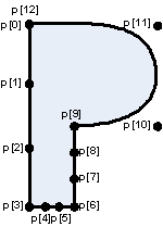Sample: Outline of character P of a scalable PostScript font composed by four consecutive cubic Bézier curves: 1: p[0], p[1], p[2], p[3] form the 1. cubic Bézier curve. Since they are collinear the left border of P is just a straight line. 2: p[3], p[4], p[5], p[6] form the 2. cubic Bézier curve. Since they are collinear the lower border of P's foot is a straight line. 3: p[6], p[7], p[8], p[9] form the 3. cubic Bézier curve. Since they are collinear the right border of P's leg is a straight line. 4: p[9], p[10], p[11], p[12]=p[0] form the 4. cubic Bézier curve. p[10] and p[11] bend the curvature. Advantage 1: Straight lines, sharp edges and curves are coded within a simple polygon. Advantage 2: Simple curves are well defined by only four vertices: p[9], p[10], p[11], p[12]=p[0]. Advantage 3: Scroll, Zoom and Rotate operations are possible as with any polygon. Disadvantage 1: Vertices p[1], p[2], p[4], p[5], p[7] and p[8] are redundant but obligatory. Disadvantage 2: A Bézier approximated polygon has to contain a certain no. of vertices: n=4 or 7 or 10 or 13 or 16 etc. Disadvantage 3: Bézier coefficients a3, a2, a1 and a0 have to be computed from any piece of 4 vertices.

Since the quadratic and cubic Bézier curves are needed by nearly all fonts, the modern microprocessors provide (very fast) micro programs to compute the quadratic Bézier coefficients a₂, a₁ and a₀ or the cubic Bézier coefficients a₃, a₂, a₁ and a₀. You can directly call the microprogram for cubic approximation in C# by DrawPolyBezier( Pen pen, PointF[] p ); where p.Length must be 4 or 7 or 10 or 13 or 16 etc.
Rational Bézier curves
Some curves like the circle cannot be described by a Bézier curve or a piecewise Bézier curve. To describe these other curves, additional degrees of freedom are offered by Rational Bézier curves. A rational Bézier curve is a fraction of two polynomials and adds adjustable weights to the vertices.

Cubic Spline Interpolation

Etymology: Spline is a shipbuilding yard word describing the bent of arbors or steel plates of the hull of a ship.
Cubic splines connect 4 vertices by polynomials of degree 3 as cubic Bézier curves do. But they have additional interesting properties.

New properties: 1. Splines hit all vertices exactly. 2. Splines avoid any discontinuity at the butt joint vertex (here: p[3]) between two polynomials. 3. Splines produce the illusion of one single polynomial of degree n-1 and hide the presence of a sequence of short single polynomials of degree 3. Sample: The 1st polynomial starts at p[0] with a selectable slope, hits p[1] and p[2] and ends at p[3]. The 2nd polynomial starts at p[3] with the slope (1. derivative) and curvature (2. derivative) of 1st polynomial's end. There is no visible discontinuity at p[3] since the 1st and 2nd derivatives of both polynomials at p[3] are identical. see: Wikipedia: Spline (mathematics)

In addition to quadratic and cubic Bézier curves, modern microprocessors provide (very fast) micro programs to compute cubic splines from polygons.
Transitions between Bézier curves and splines
Bézier curves and splines have a common mathematical basis. Any transitions between both concepts are possible by giving a weight to any vertex via Rational Bézier curves. The weight codes the traction that a vertex exercises on the curve. With high weights Rational Bézier curves behave like splines.
NURBS = Non Uniform Rational B-Splines
are generalizations of non-rational B-splines and non-rational and rational Bezier curves and surfaces and provide the flexibility to design a large variety of 2D- and 3D-shapes.

Programming curves in parametric form

In computer graphics all sorts of 2D-lines (straight, parabolas, ellipses, Bézier curves, splines etc.) are written in form of two equations with a parameter t.
Example 1: A straight line between two vertices x0,y0 and x1,y1 in parametric form:
x = x0 + t * ( x1 - x0 );
y = y0 + t * ( y1 - y0 );
where t takes any value between 0.0 and 1.0.
If you want to compute 100 points between x0,y0 and x1,y1 you just write the simple program:
float[] x = new Single[100]; float[] y = new Single[100];
for ( int i=0; i < 100; i++ )
{ float t = i * 0.01f;
  x[i] = x0 + t * ( x1 - x0 );
  y[i] = y0 + t * ( y1 - y0 );
}
Example 2: A circle with radius r and center xm,ym in parametric form:
x = xm + r * cosinus( 2 * Pi * t );
y = ym + r *   sinus( 2 * Pi * t );
where t takes any value between 0.0 and 1.0.
If you want to compute 100 points on the perimeter you just write the simple program:
float[] x = new Single[100]; float[] y = new Single[100];
for ( int i=0; i < 100; i++ )
{ double arcus = 2.0 * Math.PI * i * 0.01;
  x[i] = xm + r * (Single)Math.Cos( arcus );
  y[i] = ym + r * (Single)Math.Sin( arcus );
}

top of page: